21. Monte Carlo and Option Pricing#

21.2.1. Share price with known distribution#

Suppose that we are considering buying a share in some company.

Our plan is either to

1. buy the share now, hold it for one year and then sell it, or

2. do something else with our money.

We start by thinking of the share price in one year as a random variable $S$.

Before deciding whether or not to buy the share, we need to know some features of the distribution of $S$.

For example, suppose the mean of $S$ is high relative to the price of buying the share.

This suggests we have a good chance of selling at a relatively high price.

Suppose, however, that the variance of $S$ is also high.

This suggests that buying the share is risky, so perhaps we should refrain.

Either way, this discussion shows the importance of understanding the distribution of $S$.

Suppose that, after analyzing the data, we guess that $S$ is well represented by a lognormal distribution with parameters $\mu, \sigma$ .

• $S$ has the same distribution as $\exp(\mu + \sigma Z)$ where $Z$ is standard normal.

• We write this statement as $S \sim LN(\mu, \sigma)$.

Any good reference on statistics (such as Wikipedia) will tell us that the mean and variance are

and

So far we have no need for a computer.

21.2.2. Share price with unknown distribution#

But now suppose that we study the distribution of $S$ more carefully.

We decide that the share price depends on three variables, $X_1$, $X_2$, and $X_3$ (e.g., sales, inflation, and interest rates).

In particular, our study suggests that

where

• $p$ is a positive number, which is known to us (i.e., has been estimated),

• $X_i \sim LN(\mu_i, \sigma_i)$ for $i=1,2,3$,

• the values $\mu_i, \sigma_i$ are also known, and

• the random variables $X_1$, $X_2$ and $X_3$ are independent.

How should we compute the mean of $S$?

To do this with pencil and paper is hard (unless, say, $p=1$).

But fortunately there’s an easy way to do this, at least approximately.

This is the Monte Carlo method, which runs as follows:

1. Generate $n$ independent draws of $X_1$, $X_2$ and $X_3$ on a computer,

2. use these draws to generate $n$ independent draws of $S$, and

3. take the average value of these draws of $S$.

This average will be close to the true mean when $n$ is large.

This is due to the law of large numbers, which we discussed in LLN and CLT.

We use the following values for $p$ and each $\mu_i$ and $\sigma_i$.

n = 1_000_000
p = 0.5
μ_1, μ_2, μ_3 = 0.2, 0.8, 0.4
σ_1, σ_2, σ_3 = 0.1, 0.05, 0.2

%%time

S = 0.0
for i in range(n):
    X_1 = np.exp(μ_1 + σ_1 * randn())
    X_2 = np.exp(μ_2 + σ_2 * randn())
    X_3 = np.exp(μ_3 + σ_3 * randn())
    S += (X_1 + X_2 + X_3)**p
S / n

CPU times: user 3.67 s, sys: 0 ns, total: 3.67 s
Wall time: 3.67 s

2.229789652237379

def compute_mean(n=1_000_000):
    S = 0.0
    for i in range(n):
        X_1 = np.exp(μ_1 + σ_1 * randn())
        X_2 = np.exp(μ_2 + σ_2 * randn())
        X_3 = np.exp(μ_3 + σ_3 * randn())
        S += (X_1 + X_2 + X_3)**p
    return (S / n)

compute_mean()

2.2297518882233383

21.2.3. A vectorized routine#

If we want a more accurate estimate we should increase $n$.

But the code above runs quite slowly.

To make it faster, let’s implement a vectorized routine using NumPy.

def compute_mean_vectorized(n=1_000_000):
    X_1 = np.exp(μ_1 + σ_1 * randn(n))
    X_2 = np.exp(μ_2 + σ_2 * randn(n))
    X_3 = np.exp(μ_3 + σ_3 * randn(n))
    S = (X_1 + X_2 + X_3)**p
    return S.mean()

%%time

compute_mean_vectorized()

CPU times: user 80.3 ms, sys: 5.99 ms, total: 86.2 ms
Wall time: 85.8 ms

2.2297150888731245

Notice that this routine is much faster.

We can increase $n$ to get more accuracy and still have reasonable speed:

%%time

compute_mean_vectorized(n=10_000_000)

CPU times: user 791 ms, sys: 50 ms, total: 841 ms
Wall time: 841 ms

2.2297247427698874

21.3.1. Risk-neutral pricing#

When we use risk-neutral pricing, we determine the price of a given asset according to its expected payoff:

For example, suppose someone promises to pay you

• 1,000,000 dollars if “heads” is the outcome of a fair coin flip

• 0 dollars if “tails” is the outcome

Let’s denote the payoff as $G$, so that

Suppose in addition that you can sell this promise to anyone who wants it.

• First they pay you $P$, the price at which you sell it

• Then they get $G$, which could be either 1,000,000 or 0.

What’s a fair price for this asset (this promise)?

The definition of “fair” is ambiguous, but we can say that the risk-neutral price is 500,000 dollars.

This is because the risk-neutral price is just the expected payoff of the asset, which is

21.3.2. A comment on risk#

As suggested by the name, the risk-neutral price ignores risk.

To understand this, consider whether you would pay 500,000 dollars for such a promise.

Would you prefer to receive 500,000 for sure or 1,000,000 dollars with 50% probability and nothing with 50% probability?

At least some readers will strictly prefer the first option — although some might prefer the second.

Thinking about this makes us realize that 500,000 is not necessarily the “right” price — or the price that we would see if there was a market for these promises.

Nonetheless, the risk-neutral price is an important benchmark, which economists and financial market participants try to calculate every day.

21.3.3. Discounting#

Another thing we ignored in the previous discussion was time.

In general, receiving $x$ dollars now is preferable to receiving $x$ dollars in $n$ periods (e.g., 10 years).

After all, if we receive $x$ dollars now, we could put it in the bank at interest rate $r > 0$ and receive $(1 + r)^n x$ in $n$ periods.

Hence future payments need to be discounted when we consider their present value.

We will implement discounting by

• multiplying a payment in one period by $\beta < 1$

• multiplying a payment in $n$ periods by $\beta^n$, etc.

The same adjustment needs to be applied to our risk-neutral price for the promise described above.

Thus, if $G$ is realized in $n$ periods, then the risk-neutral price is

21.3.4. European call options#

Now let’s price a European call option.

The option is described by three things:

2. $n$, the expiry date,

3. $K$, the strike price, and

4. $S_n$, the price of the underlying asset at date $n$.

For example, suppose that the underlying is one share in Amazon.

The owner of this option has the right to buy one share in Amazon at price $K$ after $n$ days.

If $S_n > K$, then the owner will exercise the option, buy at $K$, sell at $S_n$, and make profit $S_n - K$.

If $S_n \leq K$, then the owner will not exercise the option and the payoff is zero.

Thus, the payoff is $\max\{ S_n - K, 0 \}$.

Under the assumption of risk neutrality, the price of the option is the expected discounted payoff:

Now all we need to do is specify the distribution of $S_n$, so the expectation can be calculated.

Suppose we know that $S_n \sim LN(\mu, \sigma)$ and $\mu$ and $\sigma$ are known.

If $S_n^1, \ldots, S_n^M$ are independent draws from this lognormal distribution then, by the law of large numbers,

We suppose that

μ = 1.0
σ = 0.1
K = 1
n = 10
β = 0.95

We set the simulation size to

M = 10_000_000

Here is our code

S = np.exp(μ + σ * np.random.randn(M))
return_draws = np.maximum(S - K, 0)
P = β**n * np.mean(return_draws)
print(f"The Monte Carlo option price is approximately {P:3f}")

The Monte Carlo option price is approximately 1.036937

21.4.1. Simple dynamics#

One simple model for $\{S_t\}$ is

where

• $S_0$ is lognormally distributed and

• $\{ \xi_t \}$ is IID and standard normal.

Under the stated assumptions, $S_n$ is lognormally distributed.

To see why, observe that, with $s_t := \ln S_t$, the price dynamics become

Since $s_0$ is normal and $\xi_1$ is normal and IID, we see that $s_1$ is normally distributed.

Continuing in this way shows that $s_n$ is normally distributed.

Hence $S_n = \exp(s_n)$ is lognormal.

21.4.2. Problems with simple dynamics#

The simple dynamic model we studied above is convenient, since we can work out the distribution of $S_n$.

However, its predictions are counterfactual because, in the real world, volatility (measured by $\sigma$) is not stationary.

Instead it rather changes over time, sometimes high (like during the GFC) and sometimes low.

In terms of our model above, this means that $\sigma$ should not be constant.

21.4.3. More realistic dynamics#

This leads us to study the improved version:

where

Here $\{\eta_t\}$ is also IID and standard normal.

21.4.4. Default parameters#

For the dynamic model, we adopt the following parameter values.

default_μ  = 0.0001
default_ρ  = 0.1
default_ν  = 0.001
default_S0 = 10
default_h0 = 0

(Here default_S0 is $S_0$ and default_h0 is $h_0$.)

For the option we use the following defaults.

default_K = 100
default_n = 10
default_β = 0.95

21.4.5. Visualizations#

With $s_t := \ln S_t$, the price dynamics become

Here is a function to simulate a path using this equation:

def simulate_asset_price_path(μ=default_μ, S0=default_S0, h0=default_h0, n=default_n, ρ=default_ρ, ν=default_ν):
    s = np.empty(n+1)
    s[0] = np.log(S0)

    h = h0
    for t in range(n):
        s[t+1] = s[t] + μ + np.exp(h) * randn()
        h = ρ * h + ν * randn()

    return np.exp(s)

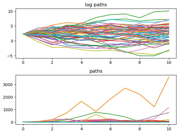
Here we plot the paths and the log of the paths.

fig, axes = plt.subplots(2, 1)

titles = 'log paths', 'paths'
transforms = np.log, lambda x: x
for ax, transform, title in zip(axes, transforms, titles):
    for i in range(50):
        path = simulate_asset_price_path()
        ax.plot(transform(path))
    ax.set_title(title)

fig.tight_layout()
plt.show()

21.4.6. Computing the price#

Now that our model is more complicated, we cannot easily determine the distribution of $S_n$.

So to compute the price $P$ of the option, we use Monte Carlo.

We average over realizations $S_n^1, \ldots, S_n^M$ of $S_n$ and appealing to the law of large numbers:

Here’s a version using Python loops.

def compute_call_price(β=default_β,
                       μ=default_μ,
                       S0=default_S0,
                       h0=default_h0,
                       K=default_K,
                       n=default_n,
                       ρ=default_ρ,
                       ν=default_ν,
                       M=10_000):
    current_sum = 0.0
    # For each sample path
    for m in range(M):
        s = np.log(S0)
        h = h0
        # Simulate forward in time
        for t in range(n):
            s = s + μ + np.exp(h) * randn()
            h = ρ * h + ν * randn()
        # And add the value max{S_n - K, 0} to current_sum
        current_sum += np.maximum(np.exp(s) - K, 0)

    return β**n * current_sum / M

%%time
compute_call_price()

CPU times: user 190 ms, sys: 1 μs, total: 190 ms
Wall time: 190 ms

1204.1987397958637